Sorting Algorithms

Introduction

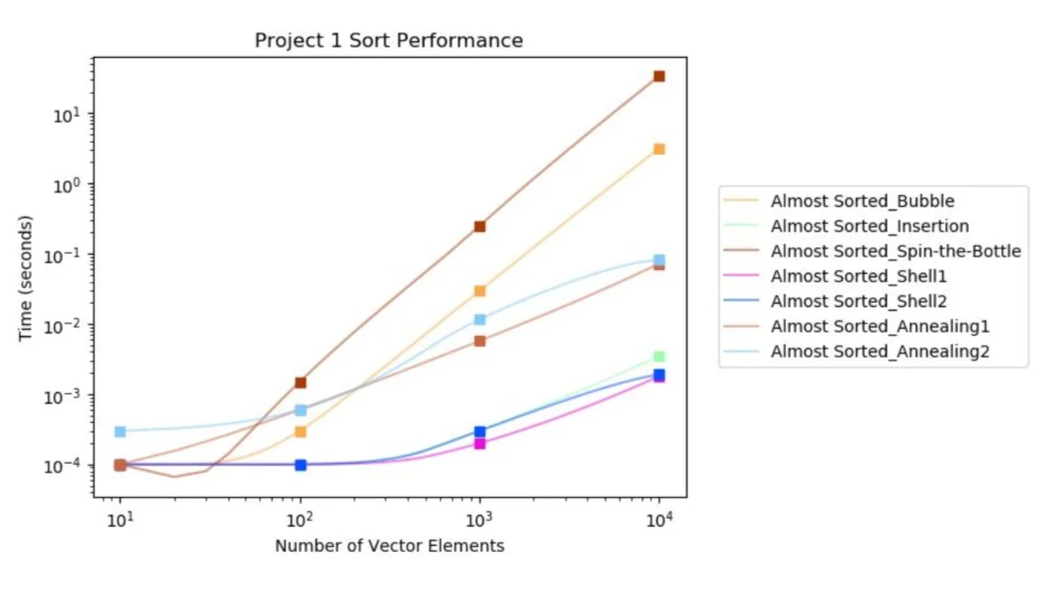
The goal for this project was to implement and analyze 5 different sorting algorithms: Bubble-sort, Insertion-sort, Spin-the-Bottle sort, Shellsort, and Annealing sort. I will discuss my implementation, run-time performance, and conclusions drawn from running these algorithms. I ran each algorithm 100 times on list with sizes n = 10, 100, 1000, 10000 and with uniformly generated and almost sorted list distributions. For my graphs, I plotted them on a “log” scale and normalized values by adding 0.0001 to assist in plotting values of zero. If I did not do this, my graphs would have weird curves, bumps, and cutoffs on the on the UnivariateSpline and it was not easy to discern any useful information with missing data points. All algorithms performed with 100% accuracy. This can be confirmed by running the main and checking the terminal test bench. Additional algorithm helper functions can be found in the alg_tools.cpp file.

Bubble-sort

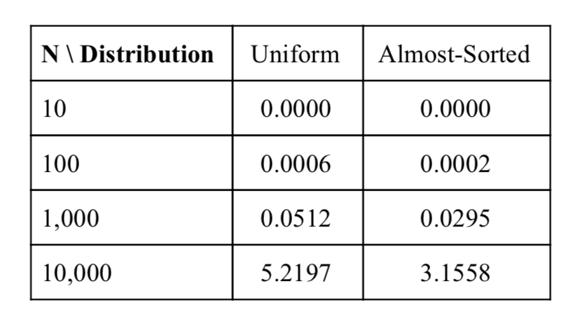
This algorithm sorts a vector of integers by repeatedly iterating through each index swapping pairs of values that are not in the correct order. This continues until there is an iteration where no values are swapped, meaning that the list is sorted. This is a very simple and relatively inefficient sorting algorithm. The worst-case running time of this algorithm is O(n^2) . Assuming that the vector is sorted in reverse order, each of the n elements will need to be checked/swapped n times in order for the entire array to be sorted. However, this is not always the case. It is also worth noting that the algorithm performs its sorting in-place and is stable. Below is the data I gathered from running my bubble-sort code. It appears that bubble-sort, on average, sorts slightly faster on almost sorted distributions. While the algorithm may have to swap less numbers on this distribution, it still may have to move values many indices and may still require many iterations on the vector. This explains why bubble-sort is not much faster on almost sorted distributions.

Insertion-Sort

Insertion-sort iterates through a vector one index at a time comparing it’s value to the previous value. This value is compared and swapped with previous values one at a time until it is in the correct place (i.e. the value before it is less than the value of the current index) before moving on to the next index in the vector. The worst case running time for this algorithm is O(n^2), but this is usually not the case in practice. Insertion-sort can run best case O(n) , linear time. In my specific implementation of insertion-sort I shift values down the list as I go, but only place the initial index once I know where it’s final location is. This saves an average of log(n) assignment operations during each iteration. Insertion sort runs much faster on almost sorted vector distributions because it has to resort a smaller set of values and does not have to reiterate, like in bubble-sort, in order to move an index many indices.

Spin-THe-Bottle Sort

This is not a very practical algorithm and is not often used in real world applications. Spin-the-bottle sort continually iterates through a vector choosing a random index from the list. If the value at the current index and the randomly chosen index are not in the correct order, they are switched. This process continues until the array is completely sorted. This algorithm has bad performance as it is randomly choosing indices and not making any intuitive assumptions about vector ordering like the other algorithms implemented. As a result of this, the algorithm has an expected run-time of O(n^2 logn) . Because of this random nature, there is little difference when running this algorithm on different vector distributions.

Shellsort

Shellsort is a variation of insertion-sort where instead of only moving an element one index at a time we check many indices ahead, determined by a gap sequence. Given this, it should be assumed that shellsort will perform better than insertion-sort. For this algorithm I tested many different gap sequences and decided on the following two gap sequences. The first is generated by the function 2^i − 1 which creates the sequence [ ..., 33, 17, 9, 5, 3, 1]. With this sequence the algorithm is expected to run in O(n^(3/2) ) worst case. The second is generated by the function 4^k + 3 * 2^(k−1) + 1 which generates the sequence [ ..., 281, 77, 23, 8, 1]. This sequence should bring the worst case running time down to O(n^(4/3) ) . The algorithm runs quickly with either sequence.

After analyzing the run performance of this algorithm, we can see that it runs much faster than insertion sort. From these observations, the two gap sequences run at roughly the same speed. However I do believe that the first gap sequence will perform much better than the second on vectors of much larger sizes. The second gap sequence has much larger gaps and may move elements too far, being counter-productive in sorting.

Annealing Sort

Similar to the previous algorithm, annealing sort depends on generated sequences of values in order to determine the final running time. Annealing sort uses a temperature and repetition sequence. I defined sequences of length 10 for my implementation. The temperature sequence defines a search range for neighboring values of an element. The repetition sequence defines how many times you should search given the current temperature. I implemented two different sets of sequences for this algorithm. The first has a temperature sequence with all values of 10, and the repetition sequence has all values of 5. This setup effectively allows any index to randomly swap with its 10 closest neighbors in a direction and repeats this 5 times. This sequence seemed to run fairly fast on this algorithm, but did not apply any intuition in finding an efficient solution. The second has a temperature sequence of [2n, 2n, n, n, n/2, n/2, ...] and a repetition sequence of values log(n)/log(log(n)). These sequences attempt to use the size of the vector to influence the behavior of the algorithm.

Based on my observations, the first sequence set performed much better than the second. I believe that the assumptions used by the second sequence set were not necessarily useful in the sorting process. In my testing of the first sequence I found that consistent small valued sequences yielded very good run-times when sorting. Additionally, sequences of decreasing repetition sizes also seemed to to work well. It appears that there does not seem to bee any considerable difference in sorting performance between vector distributions.

Conclusions

Based on my observations, the algorithms can be ordered from fastest to slowest as follows:

1. Shell sort (both sequences)

2. Annealing sort (both sequence sets)

3. Insertion sort

4. Bubble sort

5. Spin-the-Bottle sort

This is the order that I had predicted when I started working on the project. It makes sense that spin-the-bottle sort is the slowest since it uses random index comparison sorting. Bubble sort would be the next slowest because it contains on average the highest number of comparisons and swaps, causing it to have a longer run-time. Insertion sort performed much better than bubble sort, but not better than shell or annealing sort. If inefficiently implemented, both shell and annealing sort can run extremely slow. However, in my implementations they are two of the fastest algorithms. Annealing sort is the second fastest and acts as an improvement upon spin-the-bottle sort. This sorting algorithm is able to control the randomness to within a certain degree and “temper” or repeat this a few times. Because we use this intuition in our algorithm it performs very well. Finally, shellsort performs much faster than any other algorithm that I implemented. This algorithm is a direct improvement on insertion sort which already runs fairly quick.